TraceML vs torch.profiler vs cProfile

An earlier post took a ResNet-18 training run that spent almost half its GPU time waiting for the CPU to decode the next batch of images, and TraceML named it in one line: INPUT-BOUND, add workers. Three DataLoader arguments fixed it.

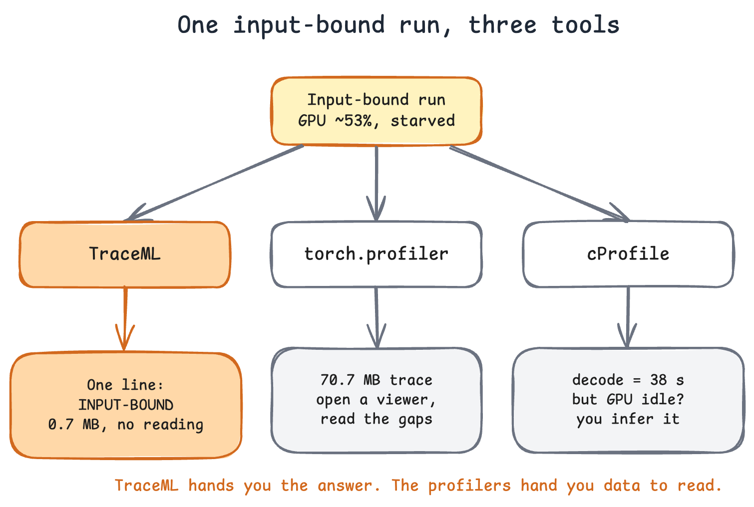
A fair question, from a torch.profiler expert's perspective: those tools find a data-loading stall too, so what does each one cost, and what do you actually do to turn its output into the same answer? This post runs all three and measures it.

The setup

The same input-bound workload as the earlier post, one T4, and the same training core under every tool, so the compute is identical and only the instrumentation changes.

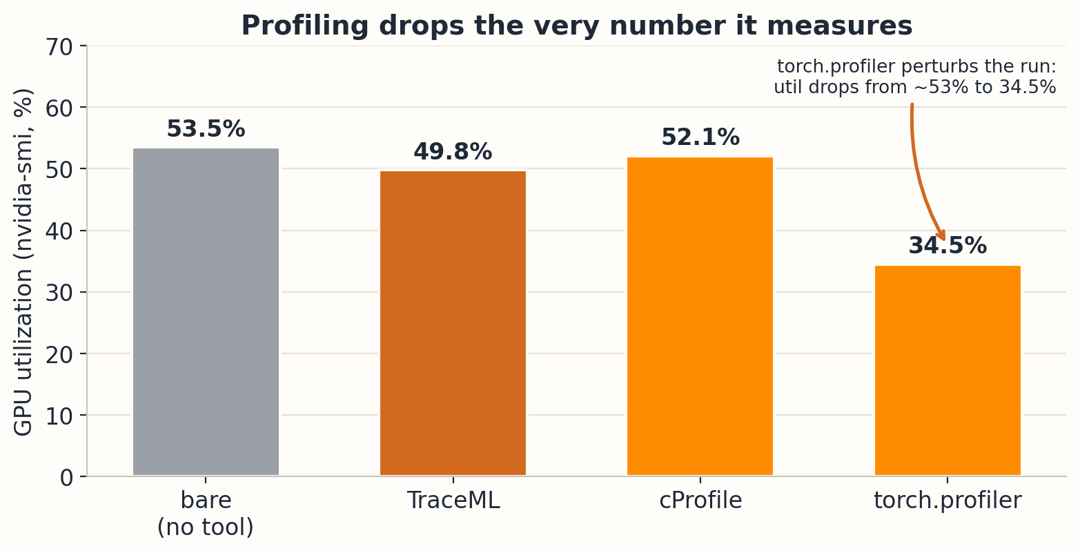
Five configurations run on it: the bare run (the wall-clock reference), TraceML, torch.profiler, cProfile, and torch.profiler and cProfile together, the pairing many engineers reach for. GPU utilization is sampled independently with nvidia-smi throughout, so no tool grades its own homework; it held around 53%, the starvation the earlier post fixed.

What each one costs

The bare run took 88.6 seconds; everything else is measured against it. One note on the Steps column: torch.profiler is built to profile a short window, so it runs 25 steps (15 profiled) rather than the full 300, and its cost is read per step.

Four numbers stand out:

• TraceML ran the whole job for an extra 1.8 seconds (+2.0%) and wrote 0.7 MB.
• cProfile added 5.9 seconds (+6.7%) across the whole run and wrote 1.6 MB.
• torch.profiler needed 24 seconds to capture a 15-step window and wrote a 70.7 MB trace, about 100 times TraceML's footprint.

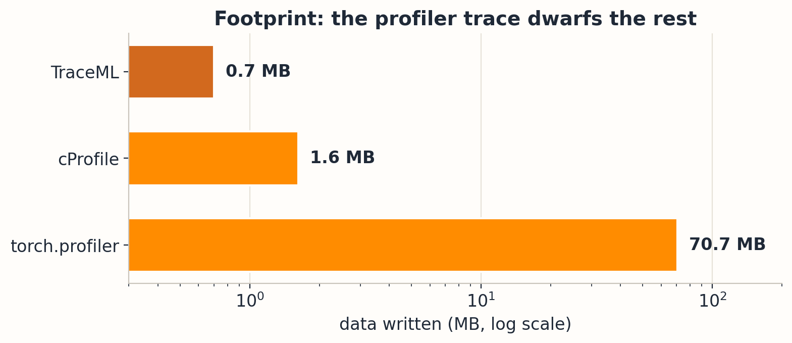
One caution on the overhead column. TraceML's 2% and cProfile's 6.7% are paid continuously, across the whole run. torch.profiler's cost is per step and only inside its short window. You would not leave it on for all 300 steps, because that trace alone would be over a gigabyte. They are not the same kind of number, which is the point of running all of them rather than one.

There is a second cost that does not show up as time or bytes. Profiling perturbs the run. While torch.profiler was capturing, the GPU utilization it was trying to measure fell from about 53% to 34.5%. The tool changes the thing it is measuring, so a short window is not just cheaper, it is also less distorted.

What it takes to run each one

The overhead column is not really where the tools differ. The effort column is. Two of them need you to change the script, run it, then open a second tool and read the output with some expertise. One does not.

• TraceML: two lines in the script, then traceml run. The verdict is written for you, live, in the terminal or an HTML report or dashboard. No reading.
• torch.profiler: wrap the loop in profile(...), call prof.step() and export_chrome_trace(), then open the 70 MB trace in Perfetto or TensorBoard and read the idle gaps.
• cProfile: python -m cProfile -o out.prof train.py, then load the .prof in pstats or snakeviz and infer the GPU consequence yourself.

All three can find it. Reading the answer is the difference.

Every tool here contains the answer. What separates them is how much work it takes to get it out.

TraceML prints this when the run ends, without being asked:

TraceML Verdict: INPUT-BOUND / CRITICAL
Why: Input wait was 124.5ms before a 172.9ms traced step.
Next: Increase workers, prefetch, or storage throughput.

The diagnosis, the evidence, and the next step are in one card.

torch.profiler produces a 70.7 MB trace.json whose events look like this:

{ "ph": "X", "cat": "cpu_op",
  "name": "autograd::engine::evaluate_function: NllLossBackward0",
  "pid": 4040, "tid": 4049, "ts": 116325, ... }

and a table of kernel names: aten::convolution_backward, volta_sgemm_128x64_nt, cudnn::winograd_nonfused. Nowhere does it say input-bound. To get there you open the trace in Perfetto or TensorBoard and read the idle gaps between GPU kernels, or you compute GPU-busy time against wall time yourself. That second path has a trap: summing per-kernel CUDA time in this run gave 1.25 times the wall window, because kernel times overlap across streams. The utilization number TraceML states plainly is one an experienced engineer can get wrong by hand.

This is why reading the profiler is a skill of its own, and why "paste the trace into an LLM and ask what is slow" has become a common shortcut. Both are the same friction.

cProfile's catch

cProfile is the interesting middle. It named the cost more precisely than anything else here:

44352   38.302   {method 'decode' of 'ImagingDecoder' objects}
19200    ...     torchvision/datasets/folder.py:260(pil_loader)
  302    ...     torch/utils/data/dataloader.py:736(__next__)   cumtime 87.8s

JPEG decoding is 38.3 seconds of a 94.5 second run. That is a sharper "why" than any phase view. But cProfile never states the consequence, that the GPU sat idle while this happened; you connect that yourself. And it only sees the decode because the loader is single-worker. Turn workers on, which is the fix, and the decode moves to child processes where cProfile in the main process is blind to it.

Where each tool belongs

The takeaway is not that one tool wins. They do different jobs.

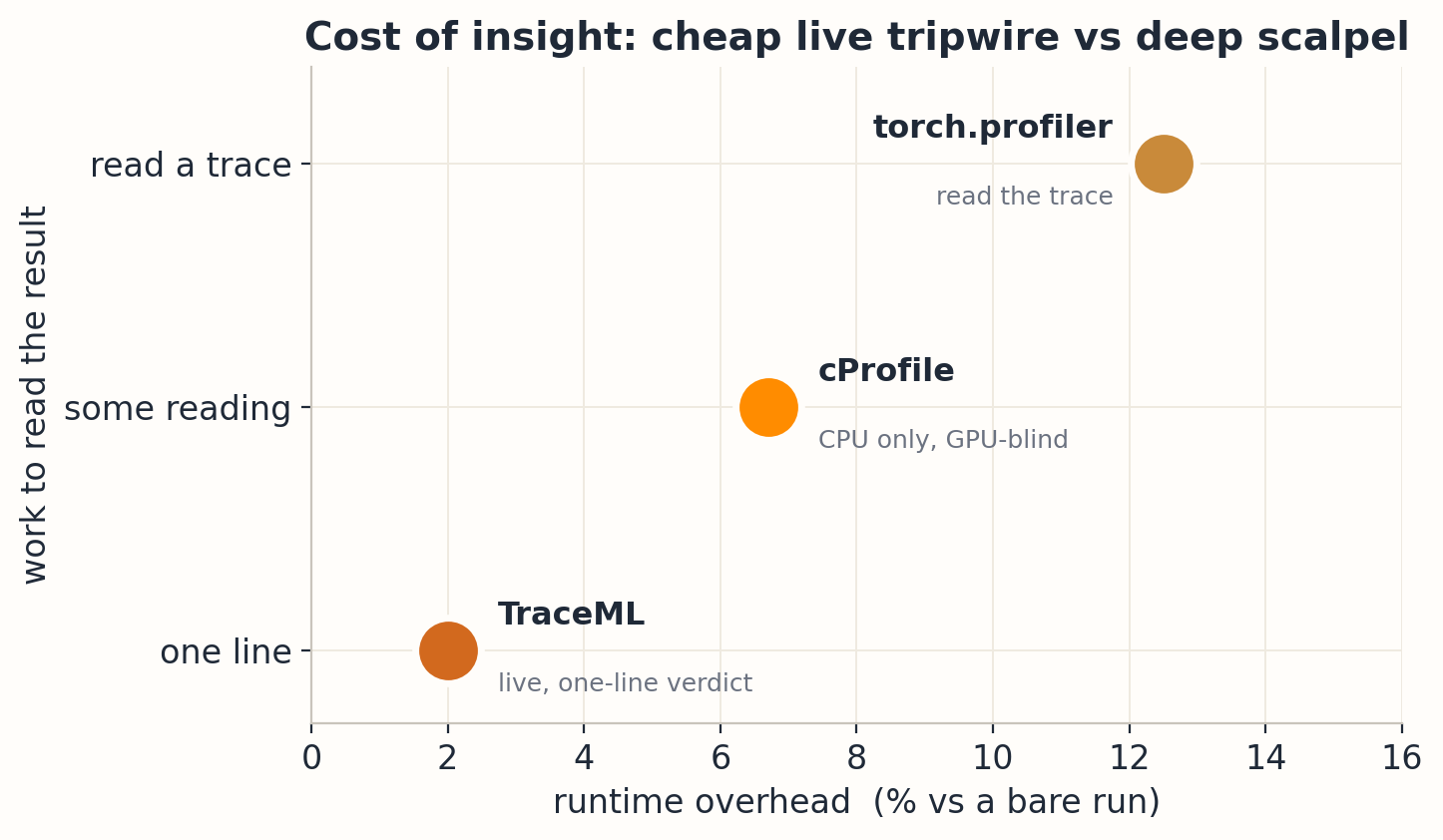
torch.profiler and cProfile are scalpels. When you already know something is slow and you need the exact kernel or the exact line, nothing else is as precise, and they work from a single step. They are the right tools for that, and TraceML does not replace them.

TraceML is the tripwire one level up. It runs live, in real time, for the whole job at 2% overhead, so a stall shows up in the numbers as it happens instead of staying invisible until you remember to profile. It will not tell you which line to change. It will tell you, on a run you never thought to profile, that you should.

Reproduce it

TraceML is open source, and the input-bound example is a short script with a companion Colab notebook.

pip install traceml-ai
traceml run --mode summary train.py \
  --args --profile baseline --max-steps 300 --batch-size 64

The torch.profiler side is the standard schedule, nothing exotic:

from torch.profiler import profile, schedule, ProfilerActivity

with profile(activities=[ProfilerActivity.CPU, ProfilerActivity.CUDA],
             schedule=schedule(wait=5, warmup=5, active=15),
             on_trace_ready=lambda p: p.export_chrome_trace("trace.json"),
             record_shapes=True, profile_memory=True) as prof:
    for images, labels in loop:
        train_step(images, labels)
        prof.step()

cProfile is a one-liner around the same script: python -m cProfile -o out.prof train.py. All the numbers above are wall-clock measurements on one T4, torch 2.11 with CUDA 13, TraceML 0.3.4, cross-checked against an independent nvidia-smi utilization trace.

The point

A correct training loop and a starved one look identical in code and in the loss curve. The only thing that separates them is where the step time goes, and you cannot see that without measuring it.

TraceML makes that first measurement cheap enough to always have. torch.profiler and cProfile make the deep read precise when you need it. The order is what matters: measure first, then profile.

Try it

Run TraceML on one real training script.

TraceML is open source and early. If you run PyTorch training, especially on rented GPUs, try it on one real training script and see whether the verdict matches your intuition.

If the summary is useful, we would love to hear what it showed. If it is wrong, confusing, or does not handle your setup cleanly, please open an issue. That feedback is the most useful thing right now.

View TraceML on GitHub Read docs

References

• Diagnosing a PyTorch DataLoader Bottleneck in a Real Training Run (the earlier post)
• PyTorch Profiler recipe
• Python cProfile documentation